Lab 9: Mapping

Orientation Control Implementation

Orientation control via the IMU’s DMP library was used to set target angles for ToF data collection. With success and high accuracy using the DMP in Lab 6, I figured that this was the best approach to ensure that the robot was reliably turning a set number of degrees throughout its rotation.

BLE and Data Transmission

The SPIN case handled initiating and running the turning logic as well as sending data over BLE at the end of collection. The case was called over bluetooth via the command: ble.send_command(CMD.SPIN, "4.6|0|0"). The parameters are used to pass through PID gains for more efficient tuning and are ordered as follows: Kp|Ki|Kd. I found that with the small changes in target angles, and the goal of moving fairly slow, that only proportional control was needed to reliably come within a degree or two of the target. At the slow speeds, there was minimal, if any, overshoot thus a derivative term was not needed. A notification handler is used to recieve the data and help pipe it into CSV files as used in previous labs.

Arduino Implementation

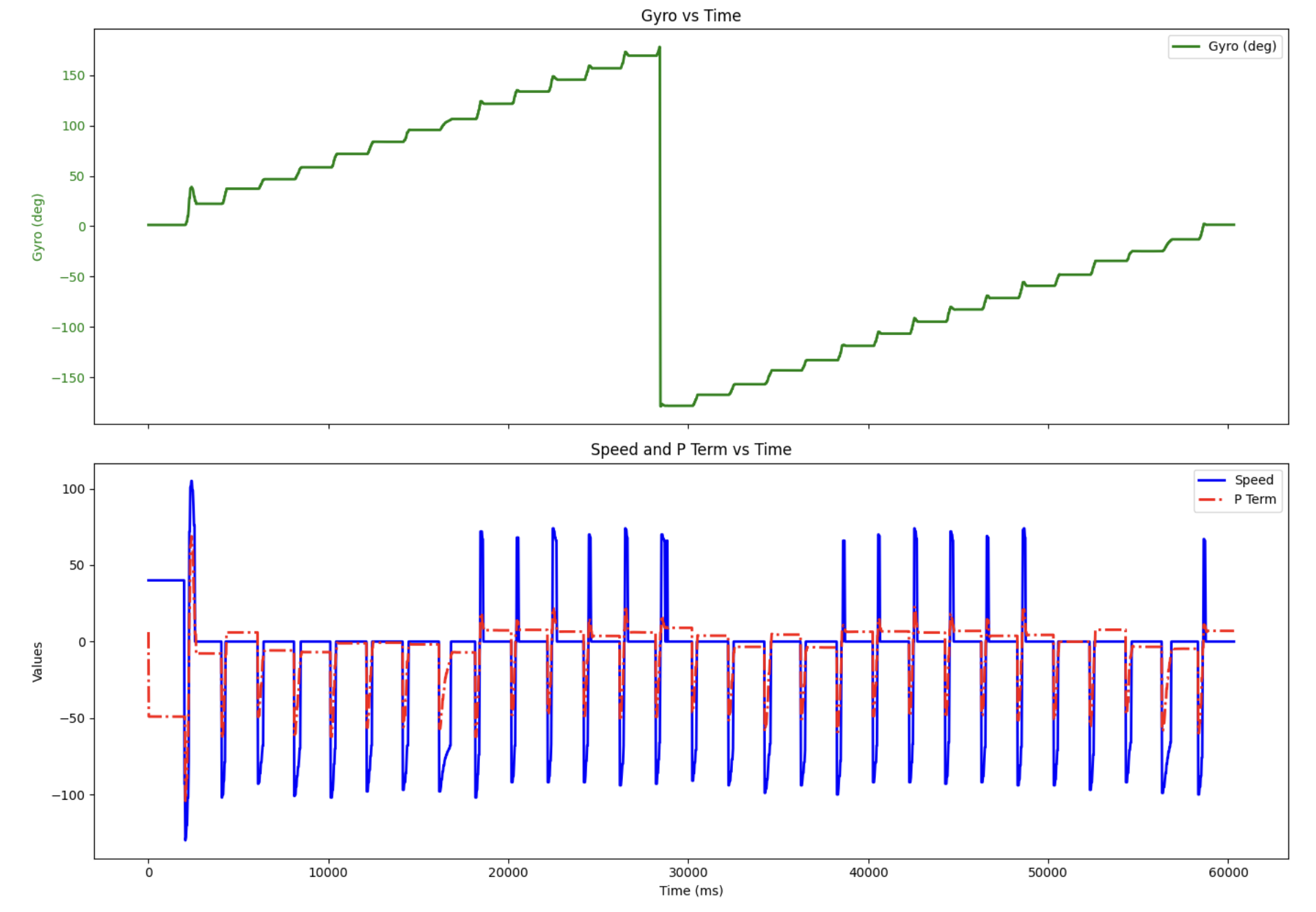
The SPIN code is shown below. The robot spins a full 360 degrees; this is broken up into 12 degrees per movement every two seconds for a total of 30 rotations. The next target angle (adding 12 to target_turn) is set every two seconds to allow for ample data collection time at a fixed angle for maximum ToF accuracy. Note that I have have ToF sensors collecting data at all times to increase the number of data points. While this does come at the cost of decreased accuracy while rotating between each two second break, it did not seem to greatly impact the ToF readings and the increased resultion was well worth the slightly decreased accuracy at a few points. Roughly 2780 ToF readings were collected per full rotation (not all necessarily unique).

distanceSensor1.startRanging();
success = robot_cmd.get_next_value(Kp_turn);
if (!success) return;
// Same for Ki and Kd

// Time varaibles
spin_time = millis();
start_time_pid_turn = millis();
last_rotation_time = millis();

while ((spin_counter < spin_len) && (rot_counter <= 30)) {
  getDMP();
  runPIDRot();
  collectTOF();
  spinTime[spin_counter] = millis() - spin_time;
  
  elapsed_time = millis() - last_rot_time;
  if (elapsed_time > 2000) {
    last_rot_time = millis();
    rot_counter = rot_counter + 1;
    target_turn = target_turn + 12;
  }   
    spin_counter = spin_counter + 1;
}
stop();
sendPIDTURNData();
break;

There are a few important functions to note, many of which have been used in my previous labs:

• getDMP() is responsible for updating the global yaw array with the current angle reading
• collectTOF() updates the global ToF arrays with the current ToF readings regardless if whether a new one is ready
• sendPIDTURNData() is responsible for sending over all relevant arrays over BLE
• runPIDRot() (shown below) is responsible for handling all rotational PID logic–it passes in the gains, target, and current angle into the pid_turn_Gyro() function which is explained in detail in Lab 6

timesROT[counter_turn] = millis() - start_time_pid_turn;

  curDistance_turn = yaw_gy;

  pidTurn_speed[counter_turn] = pid_turn_Gyro(Kp_turn, Ki_turn, Kd_turn, curDistance_turn, target_turn);

  pidTurn_p[counter_turn] = Kp_turn * pos_error_turn;
  // Same array populating for propotional, derivative, LPF derivative, and integral terms

  counter_turn = counter_turn + 1;

On-Axis Rotation Testing

Drift Error

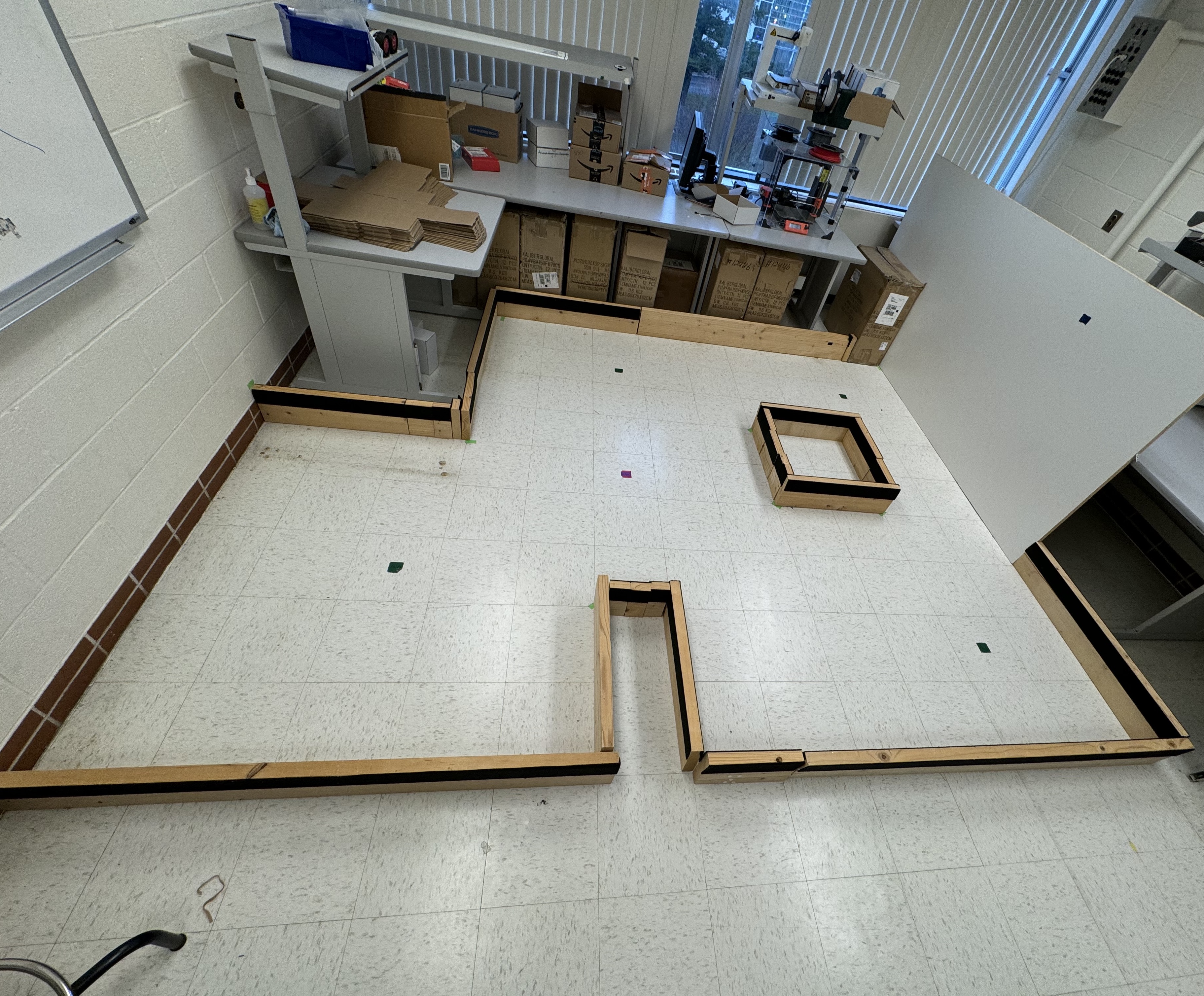
I set up a 1ft by 1ft square with a ruler in frame to test the drift of the robot over the course of the 360 degree scan. From the video you can see that the drift throughout mapping was roughly three inches likely due to wheel slip, ground friction despite wheel tape, and an inbalance of motor power. In a 4×4 meter room, this drift would not accumulate fully in one direction, but rather we can asume that it averages out across the scan point. As a result, the expected average positional error in the final map would be roughly 1.5 inches (3.8 cm). This results in a worst-case error under 1%, which is acceptable for an empty 4×4 m room. While I tried to use correction terms to reduce the drift, I was not able to completely mitigate it.

Data for Target Setting

Note you can see that for roughly 2/3 of rotations, there was no overshoot as a reverse correction input was not needed (seen on the below graph). For instances of small overshoots, they were quickly corrected as seen from a spike in speed in the opposite direction. If I wanted to completely eliminate these overshoots, I would have to make the rotations slower. This results in a memory overflow issue. The 12 degree timing every two seconds comes very close to maxing out the dynamic memory on the Artemis.

Mapping Data and Post Processing

360 Scan at Global Coordinates

For all runs, the robot was started at zero degrees facing the same way as shown in the video. The video shows a full ToF sweep taken at the coordinate (0,3)

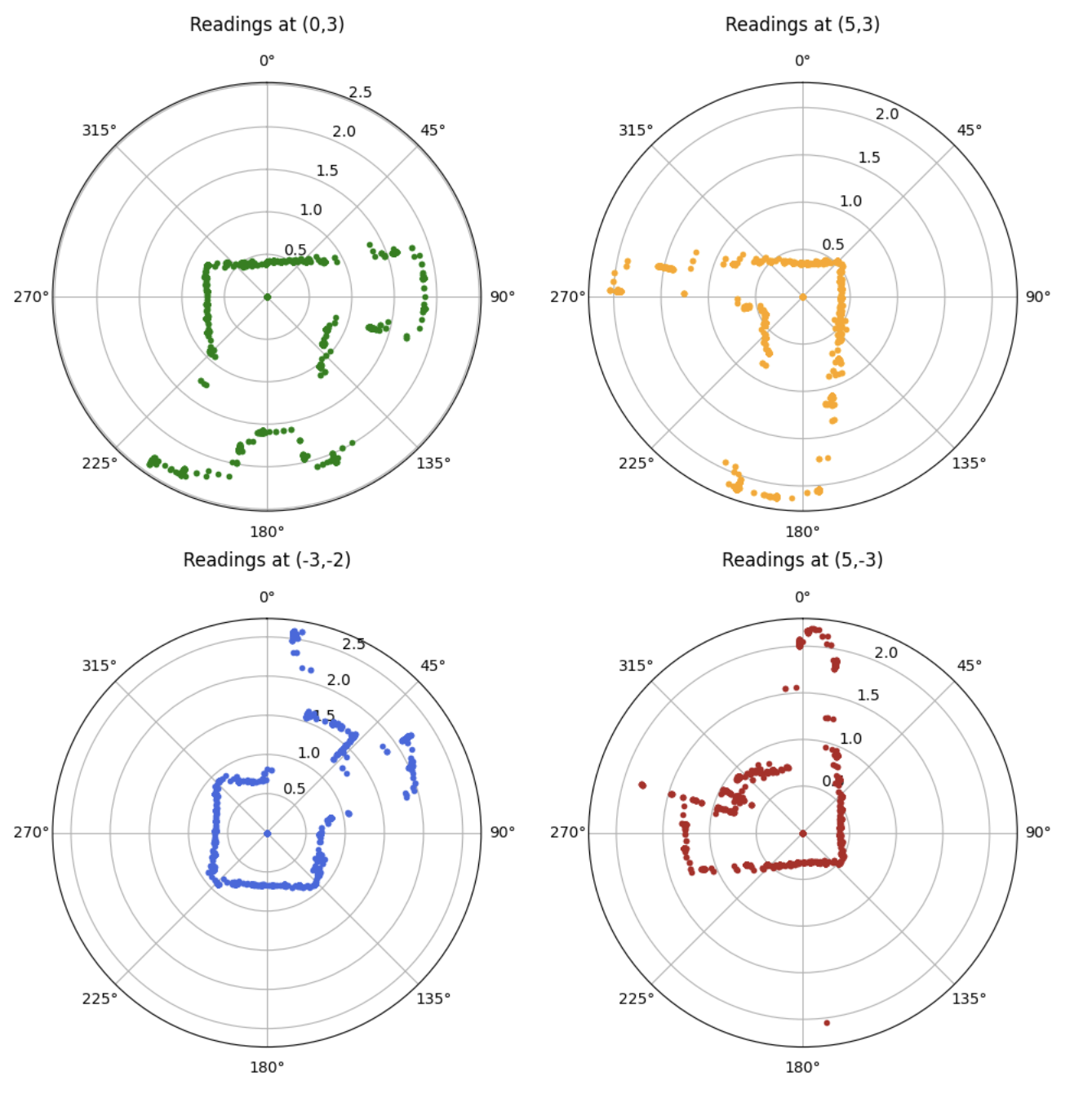
The data at each coordinate was then graphed on a polar plot for an initial sanity check

Transformation Matrices

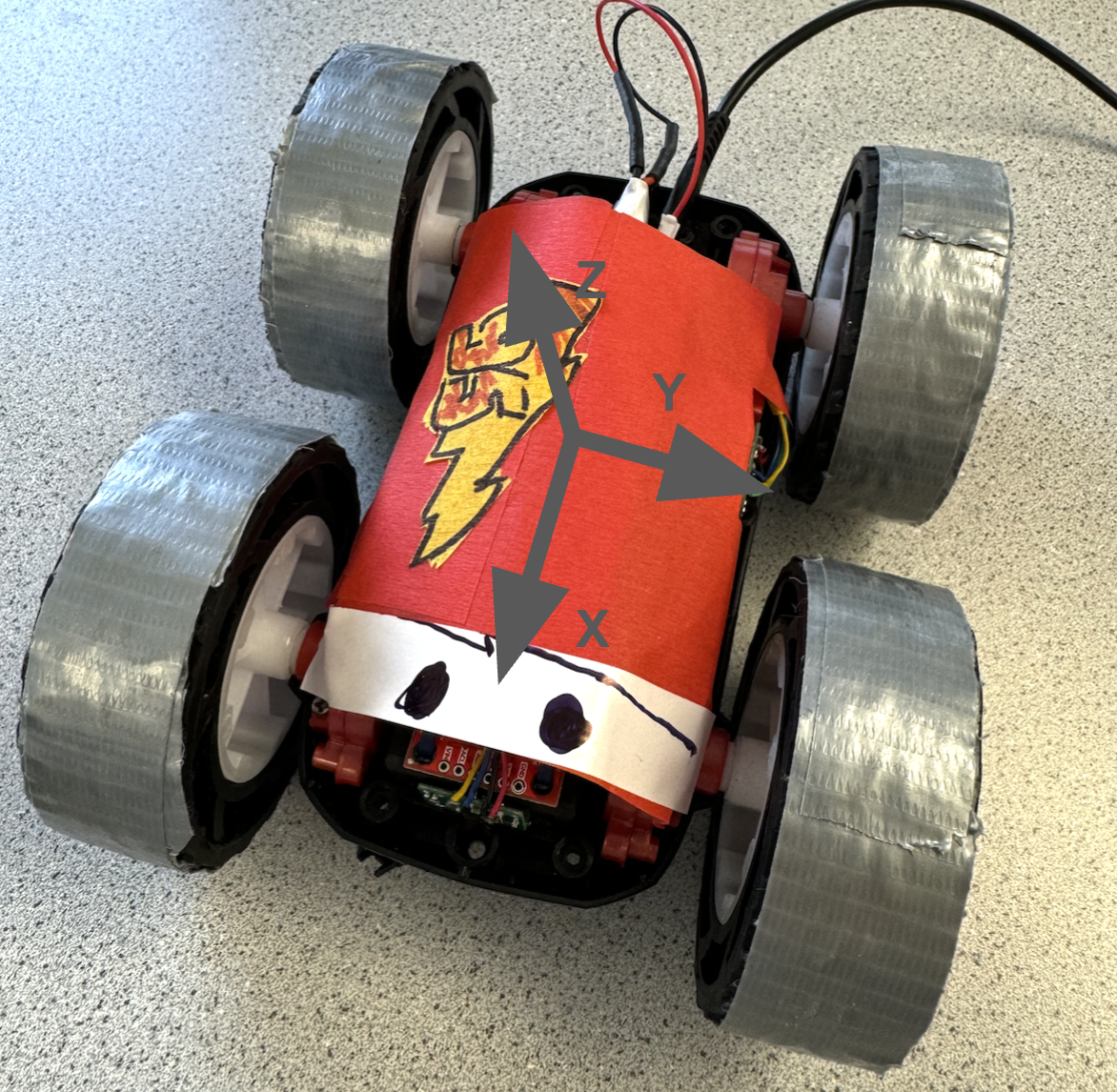
A few transformations were used to convert the raw ToF data into the global arena coordinate system. I started by taking into account the front ToF sensor location relative to the robot’s center via the robot’s coordinate axis (shown above). I found that the ToF sensor (“TOF” in the matrix) is positioned 70 mm $\hat{x}$, 0 mm $\hat{y}$ from the robots center.

The following position vector is yielded

Next, a transformation is needed to convert the robot’s local angular yaw coordinate (from the DMP) to global $\hat{x}$ and $\hat{y}$ coordinates

Map

After the transformations are applied to the raw ToF and DMP data, the following map is created

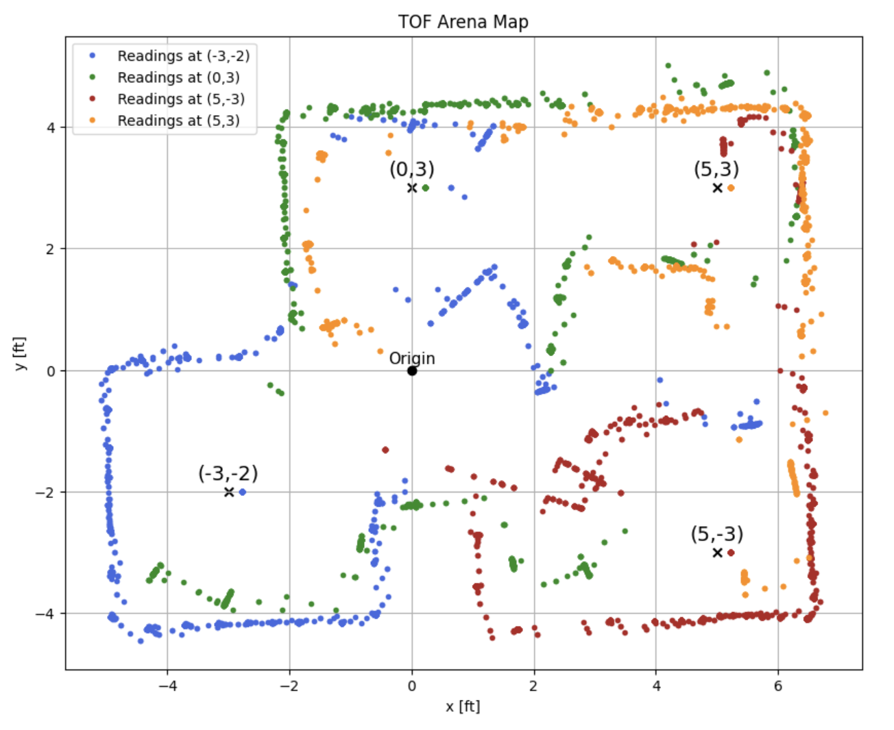
The blue arc in the middle of the arena likely indicates that a new ToF reading was not recieved for a few degrees of rotation, essentially creating part of a circle as the same ToF value is being plotted for a small sweep of angles. Additionally straight lines in the middle of the map are likely due to sensor noise as they appear in every trial.

Line-Based Map Conversion

I estimated the arena walls from the ToF map and overlayed it onto the graph. Note that some of the estimated walls appear slanted. This may be the result of a block being slightly angled at the time of data collection. The dotted black line represents the estimated arena from the ToF values

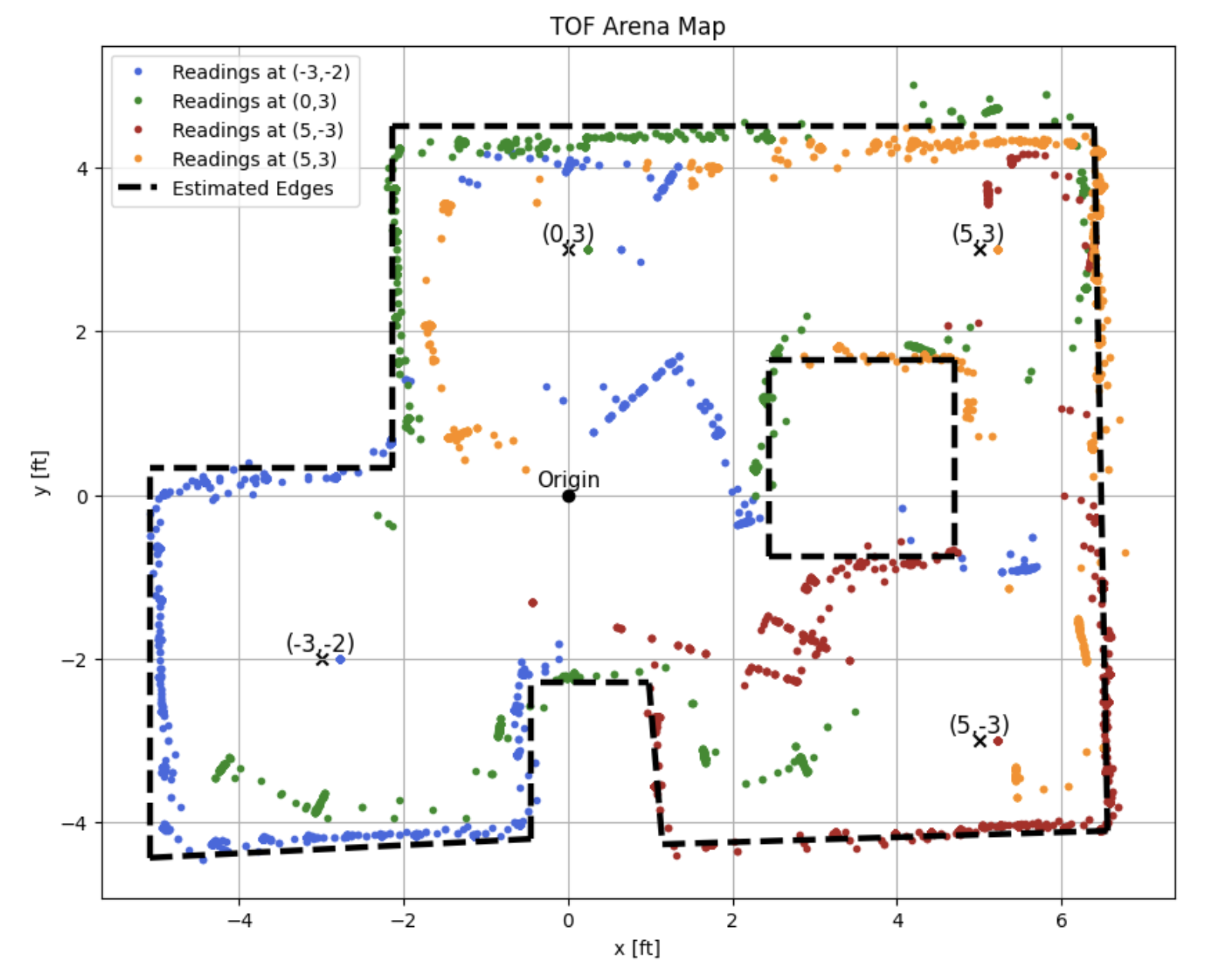
The following start and end arrays were used to create the estimated arena map (dotted black line above)

starts = [(-5.09, -4.43), (-5.09, -4.43), (-0.45, -4.2), (-0.33, -2.30), (0.98, -2.30), (1.15, -4.27), (6.56, -4.10), (6.40, 4.5), (-2.13, 4.5), (-2.13, 0.33), (2.45, 1.64), (4.7, 1.64),(4.7, -0.75), (2.45, -0.75)]

ends = [(-5.09, 0.33), (-0.45, -4.2), (-0.45, -2.30), (0.98, -2.30),(1.15, -4.27), (6.56, -4.10), (6.40, 4.5), (-2.13, 4.5), (-2.13, 0.33), (-5.09, 0.33), (4.7, 1.64), (4.7, -0.75), (2.45, -0.75), (2.45, 1.64)]

True Map

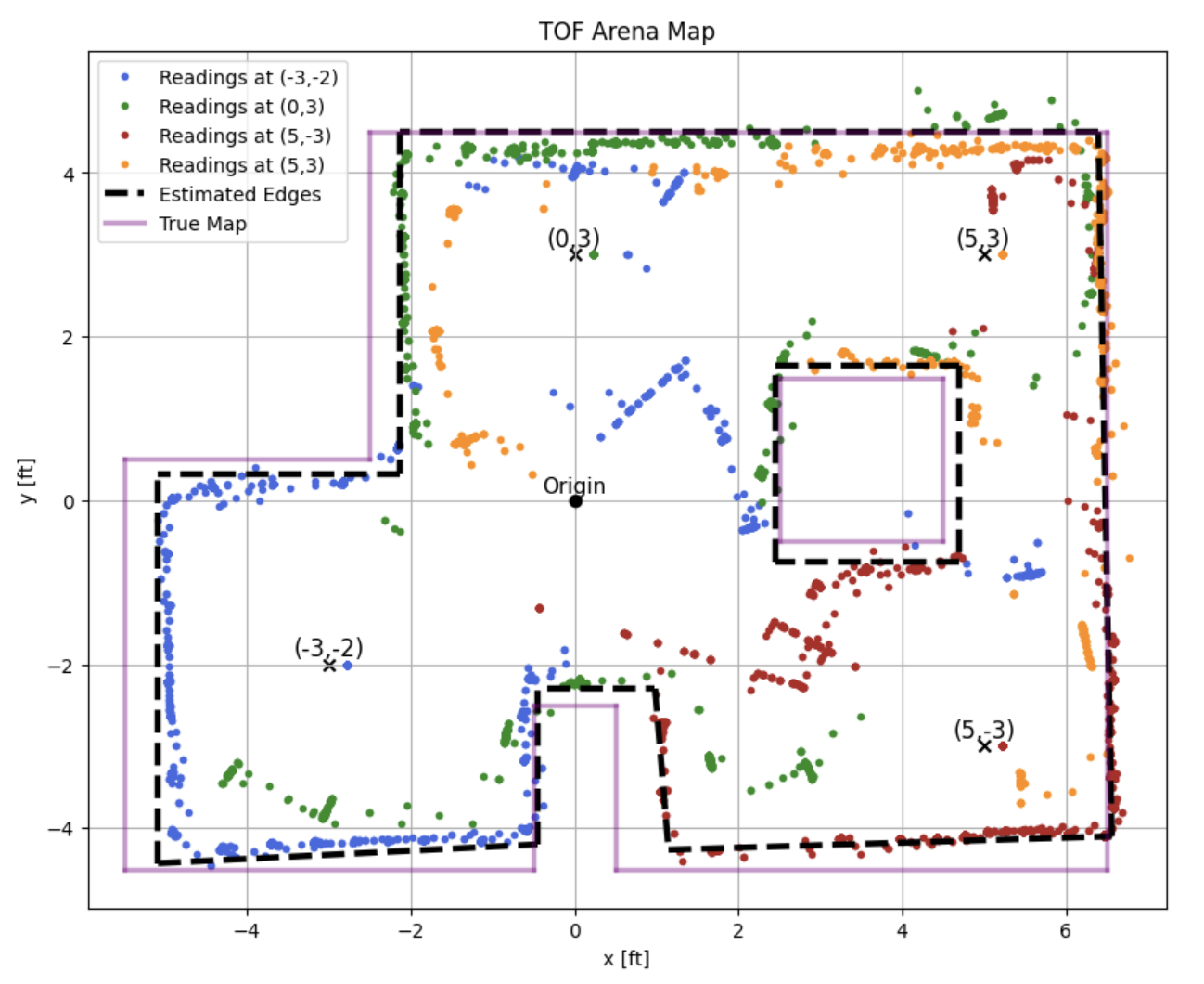
You can see that the fit between the estimated and true map are fairly close; the largest deviations appear to be at the center box and protruding wall at th bottom center. Again, I would say that this is mostly the result of ToF noise as it is constantly changing the distance away from the wall that it is seeing. Noise is especially evident when the robot is pointed at relatively far walls.

Collaboration

I collaborated extensively on this project with Jack Long and Trevor Dales. ChatGPT was used to help plot and format graphs.