Lab 10: Grid Localization using Bayes Filter
6 minutes read •
Introduction
Our robot lack absolute or “ground truth” knowledge of its position. As a result, it must infer its location using information from the environment (ToF sensors)—a process known as localization, which is most effective when approached probabilistically. To implement probabilistic localization, we use a Bayes filter, which maintains a “belief” about the robot’s position. Based on its initial state as well as ToF sensor data and control inputs, the robot forms an estimate of where it might be. As new sensor readings and inputs are received, the robot continuously updates this belief using Bayesian inference. This lab aims to implement Bayes Filter via simulation before implementing on the robot.
The robot state is 3 dimensional and is given by (x, y, $ \theta $). The robot’s world is a continuous space that spans with dimensions:
- -5.5 ft < x < 6.5 ft in the x direction
- -4.5 ft < x < 4.5 ft in the y direction
- -180°, +180° along the theta axis
The robot’s environment is represented by a grid with cells measuring 0.3048 m x 0.3048 m x 20° for a total number of cells along each axis being (12,9,18). Each cell stores the probability of the robot being in that position, with all probabilities summing to 1 to represent the robot’s belief. The Bayes filter updates these probabilities over time, and the cell with the highest probability at each step indicates the robot’s most likely pose, forming its estimated trajectory.
Bayes Filter
The Bayes filter is a iterative process that begins by estimating the robot’s next position using control inputs, and then refines this estimate based on sensor measurements. Here is the model skeleton:
Algorithm Bayes_Filter ($bel(x_{t-1}), \ u_t, \ z_t$)
for all $x_t$ do
$\overline{bel}(x_t) = \sum_{x_{t-1}} p(x_t \mid u_t, x_{t-1}) \ bel(x_{t-1})$
$bel(x_t) = \eta \ p(z_t \mid x_t) \ \overline{bel}(x_t)$
end for
return $bel(x_t)$
The prediction model can be broken down into two main parts:
- Prediction Step: the robot estimates its current position based on its previous pose and control inputs
- Update Step: this is the correction step of the Bayes Filter, where the predicted belief and sensor liklihoods are incorperated to decreases the uncertainty in the robot’s position.
Odometry Motion Model
For our purpose, control input u is expressed via an Odometry Motion Model which describes the difference between two positions or “poses”. This difference is composed of three parameters: an initial rotation, a translation, and a final rotation.
Algorithm Implementation
The following functions were used as the logic and implementation for the Bayes filter
Compute Control
The compute_control() function takes two paramenters: current pose and a previous pose. From the parameters it determines the initial rotation, translation, and final rotation which are sufficient to reconstruct the relative motion between two robot states.
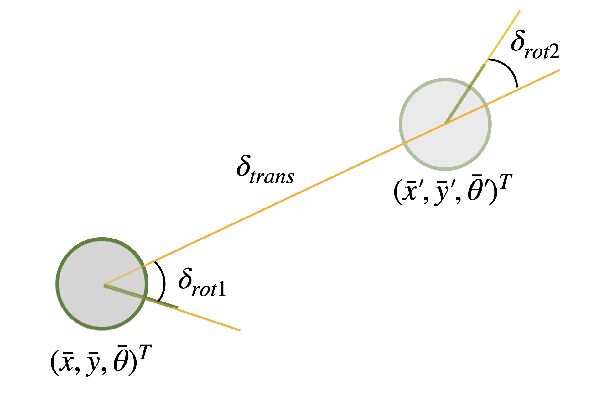
Below are the equations and code used to calculate and return the rotations and translation
$\delta_{rot1} = \text{atan2}(\bar{y}’ - \bar{y}, \bar{x}’ - \bar{x}) - \bar{\theta}$
$\delta_{trans} = \sqrt{(\bar{y}’ - \bar{y})^2 + (\bar{x}’ - \bar{x})^2}$
$\delta_{rot2} = \bar{\theta}’ - \bar{\theta} - \delta_{rot1}$
# Extract x, y, and yaw (prev and cur)
, , =
, , =
# Calculate translation in x and y and straight-line
= -
= -
=
# Rotation
= - # First rotation: from previous heading to direction of movement
= - # Final rotation: from direction of movement to current heading
# Normalize rotations [-180, 180]
=
=
return , ,
Odometry Motion Model
The odom_motion_model() function takes in a current pose and a previous pose and is responsible for predicting the probability of where a robot might be after applying noisy motion commands. Extracting the current pose, previous pose, and actual vs. predicted control inputs via compute_control(), it calculates the probabilities density of those parameters as Gaussian distributions passing in the standard deviations for rotation and translation noise.
, , =
=
=
=
= * *
return
Prediction Step
The prediction_step() function estimates the robot’s predicted belief by applying the odometry motion model to account for movement uncertainty. It takes the current and previous odometry readings, extracts control parameters, and iterates over all possible previous and current poses within the discretized 3D state space (x, y, θ). For each possible transition, it calculates the probability of moving from a previous pose to a current pose using odom_motion_model(). These probabilities are accumulated to form a predicted belief (bel_bar), which is then normalized to maintain a valid probability distribution.
To improve computational efficiency, prediction_step() skips previous states with extremely low probabilities (below 0.0001) since they contribute negligibly to the final belief. This trade-off sacrifices a small amount of accuracy and completeness in favor of significantly faster execution.
# Control input tuple
=
# Initialize belief grid
=
# Iterate over all prior belief states
=
# Skip smaller probabilities
continue
# Convert previous index to pose
=
# Iterate over all possible current states
=
# Motion model: P(cur_pose | prev_pose, u)
=
+= *
# Normalize
/=
Sensor Model
The robot’s sensors are assumed to have Gaussian noise in their readings. The sensor_model() function, like the odometry motion model, calculates the likelihood of data but based on sensor measurements instead of movement. It essentially takes a set of sensor observations at a given pose and returns the probability of receiving those observations.
=
# Calculate the likelihood of each sensor reading
=
return
Update Step
Finally, the update_step() function loops through the current state grid, calls the sensor_model() to obtain sensor likelihoods, and updates the belief accordingly. The updated belief is then normalized to ensure it sums to 1.
The below equation expresses how to calculate the total likelihood of a full set of sensor measurements zₜ given a robot’s pose xₜ and map m.
$$ p(z_t \mid x_t, m) = \prod_{k=1}^{18} p(z_t^k \mid x_t, m) $$
# Loop through all poses (x, y, theta)
# Get expected sensor reading at this pose
=
# Compare actual vs expected using the sensor model
= # p is array of individual sensor probabilities
# Update belief using product of individual sensor likelihoods
=
# bel(x) = bel_bar(x) * p(z|x)
= *
# Normalize final belief
/=
Simulation
The video below shows the shows a trajectory and localization simulation using the Bayes filter. The trajectory is pre-planned to move around the box. Here, the odometry model is plotted in red while the ground truth tracked by the simulator is plotted in green. From the video you can see the inaccuracy of the odometry model when operating in isolation.
The probabilistic belief is plotted in blue which you can see is a very good approximation of the robot’s true position. The probability distribution is also shown using the white boxes where stronger shades of white represent stronger probabilities. Note that we ignored all cells with probability <0.0001.
Notice that the initial estimation before a new sensor value is based on the odemetry model which makes sense. I also found that The Bayes Filter seems to perform better when the robot is near walls. This is likely due to the sensors being more accurate and consistent at sensing closer distances, and therfore more trustworthy. On the other hand, when it is in more open spaces such as the center of the map, the filter is slightly less accurate.
Collaboration
I collaborated extensively on this project with Jack Long and Trevor Dales. I referenced Stephan Wagner’s site for help with implementing the Bayes Filter. ChatGPT was used to help answer Bayes Filter implementation questions and conceptual misunderstandings.